SAT Collision Detection (Separating Axis Theorem): How It Works, Why It Works, and How to Implement It

SAT (Separating Axis Theorem) is one of the most practical tools in real-time collision detection. It’s fast, robust for convex shapes, and it gives you more than a boolean result: with a small extension it can also produce a penetration depth and a collision normal suitable for resolution.

This post focuses on 2D convex polygons (boxes, triangles, arbitrary convex hulls), with notes on circles and performance near the end.

Prerequisites + assumptions (read this first)

Shapes:

• Convex polygons only (or decompose concave shapes into convex pieces).
• Polygons are simple (non-self-intersecting) and have no duplicate consecutive vertices.
• Vertices are provided in consistent winding (typically CCW). SAT itself doesn’t require CCW for correctness, but consistent winding helps you compute consistent normals and debug.

Collision definition:

• Decide whether touching counts as collision.
  • If touching counts: treat overlap $\ge 0$ as contact.
  • If touching does not count: require overlap $> 0$.
• In practice you almost always use an epsilon tolerance (covered later).

Coordinate space:

• SAT is usually run on world-space vertices. If bodies rotate, cache transformed vertices/normals per frame.

Roadmap

1. Core idea: separation by projection
2. Why it works (hyperplane separation → supporting lines)
3. Projection math (dot products → intervals)
4. Worked numeric example (one axis, real numbers)
5. Implementation (polygon vs polygon) + MTV
6. Practical implementation details (epsilon, normalization, degenerate edges)
7. Extending SAT to circles (circle–circle, polygon–circle)
8. Performance notes
9. Common bugs checklist

The core idea: separation by projection

Two convex shapes do not intersect if you can find a separating line between them. In SAT we don’t search over all possible lines directly. Instead we test an axis, meaning a direction vector (usually a unit direction) $\hat{\mathbf{a}}$, and project both shapes onto that direction.

• A separating line is a geometric line in 2D space.
• A separating axis is the normal direction of some separating line.

If you project both shapes onto the same axis direction and the resulting 1D intervals do not overlap, then the shapes are separated.

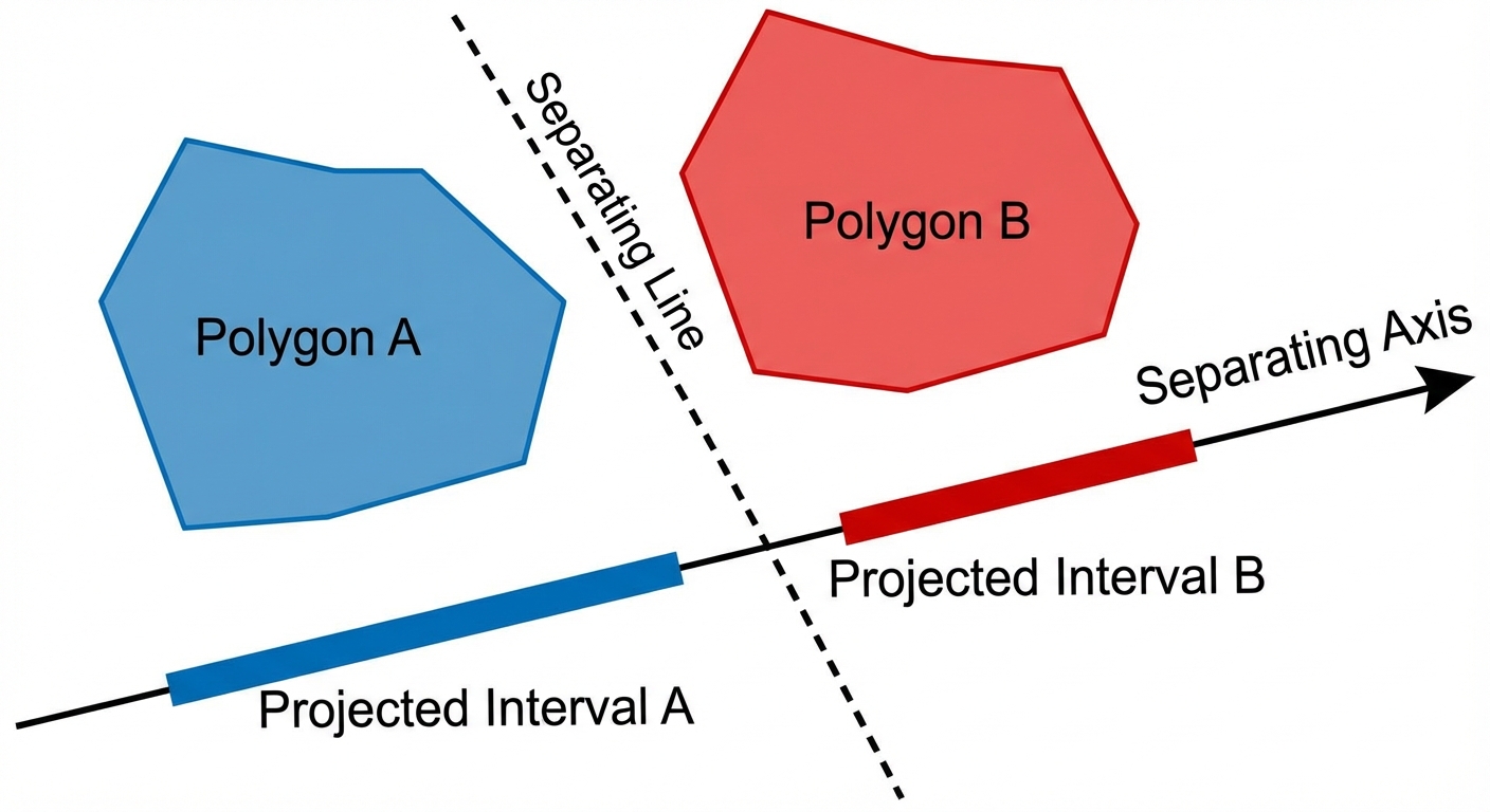
In SAT we test a finite set of candidate axes. If any axis produces non-overlapping projections, we’ve found a separating axis → no collision. If all tested axes overlap → collision.

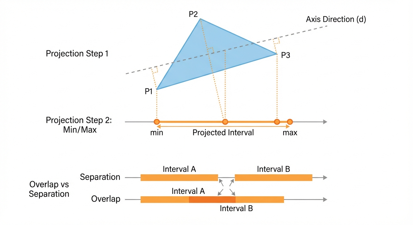
A quick overlap callout (separated vs contact)

For two projected intervals, define:

• If overlap < 0: there is a gap between intervals → shapes are separated.
• If overlap = 0: intervals just touch → shapes are in contact (whether that counts as “collision” is your definition).
• If overlap > 0: intervals overlap → shapes overlap along that axis.

This sets up why we often use an epsilon later: tiny negative overlaps can be floating-point noise.

Why it works (the theorem, intuition-first)

For convex shapes in 2D, the hyperplane separation theorem implies:

• If two convex sets are disjoint, there exists a line that separates them.

So if two convex polygons do not intersect, some separating line exists. SAT’s job is to find a normal direction for such a line.

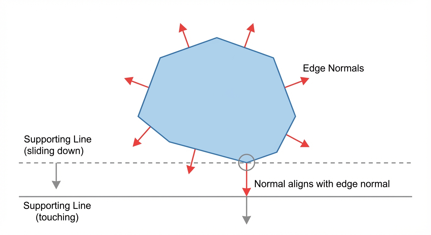
Why edge normals are enough for polygons

If a separating line exists, you can “slide” it (without rotating it) until it first touches one polygon without crossing it. At that point it becomes a supporting line of that polygon.

For a polygon, a supporting line touches the polygon at a feature:

• often an edge (line coincident with that edge), or
• sometimes a vertex.

Crucially:

• If it touches an edge, the line’s normal is exactly an edge normal.
• If it touches at a vertex, the separating direction is still captured by one of the adjacent edge normals (intuitively: the vertex is the intersection of two supporting half-planes, and the “most separating” direction aligns with a boundary direction from one of those edges).

Therefore, for polygon–polygon SAT, it’s sufficient to test the normals of all edges from both polygons.

Two important practical notes:

• You must test both polygons’ edge normals. The separating axis could come from polygon A’s edges or polygon B’s edges.
• Parallel edges create duplicate axes. Testing duplicates is correct but can be slower; deduplication is an optional optimization.

Projection math: from 2D points to a 1D interval

Pick an axis direction (a vector) $\mathbf{a}$. In implementation, you usually work with a unit axis $\hat{\mathbf{a}}$ so that overlaps are measured in world units.

Given a point $\mathbf{p}$, its scalar projection onto the axis direction is the dot product:

$\text{proj}(\mathbf{p}, \hat{\mathbf{a}}) = \mathbf{p} \cdot \hat{\mathbf{a}}$

For a polygon with vertices $\{\mathbf{v}_i\}$, the projection interval is:

• $a_{\min} = \min_i (\mathbf{v}_i \cdot \hat{\mathbf{a}})$
• $a_{\max} = \max_i (\mathbf{v}_i \cdot \hat{\mathbf{a}})$

Two intervals overlap iff:

• $a_{\max} \ge b_{\min}$ and $b_{\max} \ge a_{\min}$

And the overlap amount is:

Normalization (important, early)

• Boolean SAT (hit / no hit) works even if axes are not normalized, because dot products on both shapes scale consistently.
• MTV depth in world units requires unit axes.
  • Either normalize each axis, or
  • if using a non-unit axis $\mathbf{a}$, convert by: $\text{depthWorld} = \text{overlap} / \|\mathbf{a}\|$.

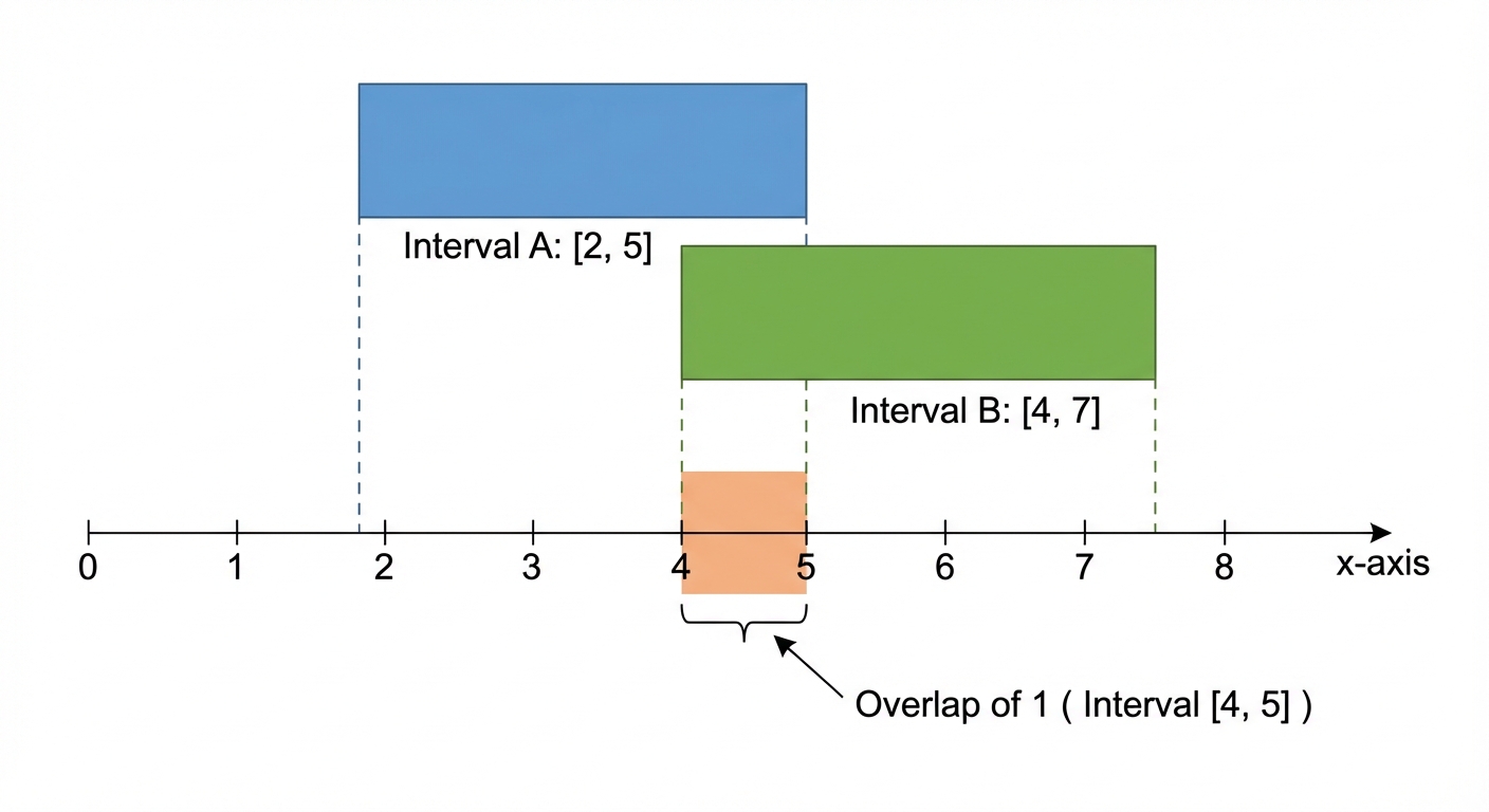
Worked example (numbers make it click)

Take two rectangles projected onto the x-axis (so $\hat{\mathbf{a}} = (1, 0)$).

• Rectangle A spans x from 2 to 5 → interval $[2, 5]$
• Rectangle B spans x from 4 to 7 → interval $[4, 7]$

Compute overlap:

So along the x-axis they overlap by 1 unit.

• If instead B were $[6, 7]$, then overlap would be $\min(5,7) - \max(2,6) = 5 - 6 = -1$ → separated.

Implementation plan (convex polygon vs convex polygon)

At a high level:

1. Build the list of candidate axes (edge normals from both polygons).
2. For each axis:
   • project both polygons
   • compute interval overlap
   • early out if separated
3. If all axes overlap, collision is true.
4. Optionally track the axis with the minimum overlap to compute the Minimum Translation Vector (MTV) for resolution.

Step 1: generate candidate axes

Given polygon vertices in order: $v_0, v_1, ..., v_{n-1}$.

Edges are:

• $e_i = v_{i+1} - v_i$ (wrapping around)

A perpendicular (normal direction) can be:

• $n_i = ( -e_i.y,\ e_i.x )$

Normalize to get a unit axis $\hat{n}_i$ if you want depth in world units.

Step 2: project a polygon onto an axis

For each vertex, compute dot products with the axis direction and track min/max.

Step 3: test overlap and early-out

For each axis:

• compute $[a_{\min}, a_{\max}]$ for polygon A
• compute $[b_{\min}, b_{\max}]$ for polygon B
• compute overlap
• if overlap is negative (or less than an epsilon threshold), you found a separating axis → return no collision

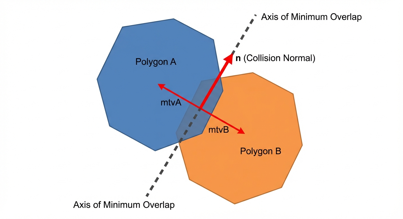
Step 4 (optional): compute MTV (collision normal + depth)

If you want resolution, keep the smallest overlap across all axes:

• $\text{depth} =$ smallest overlap
• $\text{normal} =$ axis corresponding to smallest overlap

You also need a consistent direction for the normal (e.g., from A to B). A common approach:

• compute a direction vector between shape “centers”
• if $(c_B - c_A) \cdot normal < 0$, flip the normal

Sign convention (make it explicit):

• Let normal point from A to B.
• Then the MTV that moves A out of B is:

and the MTV that moves B out of A is:

Reference implementation (TypeScript-like pseudocode)

This is intentionally “engine-agnostic” and focuses on clarity. It also guards against common edge cases (empty arrays, degenerate edges), and uses a consistent MTV convention.

type Vec2 = { x: number; y: number };

type Interval = { min: number; max: number };

type SATResult =
  | { hit: false }
  | { hit: true; normal: Vec2; depth: number; mtvA: Vec2; mtvB: Vec2 };

const EPS = 1e-9;

function add(a: Vec2, b: Vec2): Vec2 { return { x: a.x + b.x, y: a.y + b.y }; }
function sub(a: Vec2, b: Vec2): Vec2 { return { x: a.x - b.x, y: a.y - b.y }; }
function scale(v: Vec2, s: number): Vec2 { return { x: v.x * s, y: v.y * s }; }
function dot(a: Vec2, b: Vec2): number { return a.x * b.x + a.y * b.y; }
function perp(e: Vec2): Vec2 { return { x: -e.y, y: e.x }; }
function len(v: Vec2): number { return Math.hypot(v.x, v.y); }

function normalize(v: Vec2): Vec2 {
  const l = len(v);
  if (l <= EPS) return { x: 0, y: 0 };
  return { x: v.x / l, y: v.y / l };
}

// Not the true area centroid; good enough to choose a consistent normal direction in many games.
function centerOfVertices(verts: Vec2[]): Vec2 {
  let c = { x: 0, y: 0 };
  for (const v of verts) c = add(c, v);
  return scale(c, 1 / verts.length);
}

function projectPolygon(verts: Vec2[], axisUnit: Vec2): Interval {
  let min = dot(verts[0], axisUnit);
  let max = min;
  for (let i = 1; i < verts.length; i++) {
    const p = dot(verts[i], axisUnit);
    if (p < min) min = p;
    if (p > max) max = p;
  }
  return { min, max };
}

function intervalOverlap(a: Interval, b: Interval): number {
  return Math.min(a.max, b.max) - Math.max(a.min, b.min);
}

function polygonAxes(verts: Vec2[]): Vec2[] {
  const axes: Vec2[] = [];
  for (let i = 0; i < verts.length; i++) {
    const j = (i + 1) % verts.length;
    const edge = sub(verts[j], verts[i]);
    const axis = normalize(perp(edge));
    // Skip degenerate edges
    if (Math.abs(axis.x) > EPS || Math.abs(axis.y) > EPS) axes.push(axis);
  }
  return axes;
}

export function satPolygonPolygon(aVerts: Vec2[], bVerts: Vec2[]): SATResult {
  // Guard against invalid input
  if (aVerts.length < 3 || bVerts.length < 3) return { hit: false };

  const axes = [...polygonAxes(aVerts), ...polygonAxes(bVerts)];
  if (axes.length === 0) return { hit: false };

  let minDepth = Infinity;
  let bestAxis: Vec2 | null = null;

  for (const axis of axes) {
    const aProj = projectPolygon(aVerts, axis);
    const bProj = projectPolygon(bVerts, axis);

    const o = intervalOverlap(aProj, bProj);

    // Treat tiny negative as contact if you want "touching counts"
    if (o < -EPS) return { hit: false }; // separating axis found

    // Prefer smallest overlap; add a small bias to reduce axis-flip jitter
    if (o < minDepth - EPS) {
      minDepth = o;
      bestAxis = axis;
    }
  }

  if (!bestAxis || !isFinite(minDepth)) return { hit: false };

  // Ensure normal points from A to B
  const dir = sub(centerOfVertices(bVerts), centerOfVertices(aVerts));
  let normal = bestAxis;
  if (dot(dir, normal) < 0) normal = scale(normal, -1);

  const depth = Math.max(0, minDepth); // clamp tiny negatives to 0 contact

  // Convention:
  // - normal points A -> B
  // - mtvA moves A out of B
  // - mtvB moves B out of A
  const mtvB = scale(normal, depth);
  const mtvA = scale(normal, -depth);

  return { hit: true, normal, depth, mtvA, mtvB };
}

Practical details that matter in real projects

Epsilon and “touching” behavior

In games, “touching” often counts as collision/contact. With floating point error, you usually want:

• separated if overlap < -EPS
• contact/collision otherwise

Choose EPS relative to your world scale. If your coordinates are large (e.g., thousands), consider a larger EPS or a scale-aware EPS.

Normalization recap (boolean vs MTV)

• If you normalize axes, your depth is already in world units.
• If you don’t normalize axes, boolean SAT still works, but your depth is scaled by $\|\mathbf{a}\|$ and must be corrected.

Degenerate edges and duplicate vertices

Zero-length edges (often from duplicate consecutive vertices) produce a zero axis. Skip them, and ensure you don’t accidentally select a zero axis as bestAxis.

Precision note (far from origin)

Dot products can lose precision when coordinates are very large. JavaScript uses double precision, which helps, but you can still see jitter:

• keep your simulation near the origin when possible (floating origin)
• use EPS that matches your scale
• avoid unnecessary subtract/add of huge numbers

Axis deduplication tradeoffs

Deduplicating axes can speed up rectangles and simple hulls, but it’s easy to do incorrectly:

• canonicalization (e.g., force axis to a half-plane) requires an epsilon
• if your epsilon is too large, you might collapse near-parallel but distinct axes (bad for skinny polygons)

Correctness does not require deduplication.

World-space transforms (practical tip)

SAT is usually run on world-space vertices. For rotating bodies:

• transform local vertices to world once per frame
• reuse the transformed list for all collision pairs that frame

Extending SAT to circles (and polygon vs circle)

SAT is primarily a convex polytope method, but circles fit nicely.

Circle vs circle

One axis: the line between centers.

• Collision when distance $\le r_1 + r_2$.

Polygon vs circle

Test polygon edge normals as usual, plus one more axis:

• the axis from the circle center to the closest point on the polygon boundary (closest point on any edge segment)

This extra axis is crucial because the “most separating” direction can point toward a vertex region, not perpendicular to any edge.

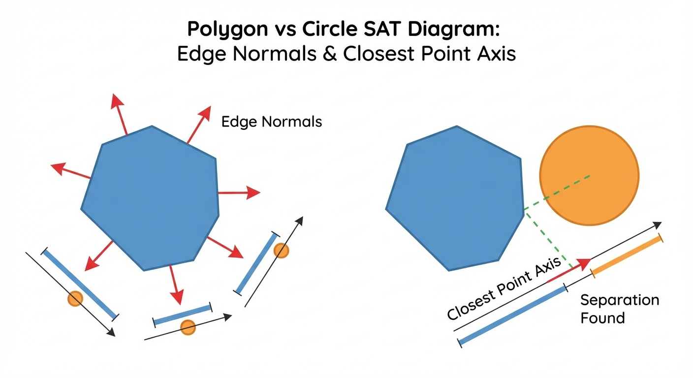
Implementation sketch:

• compute closest point on each polygon edge segment to the circle center; keep the closest
• axis = normalize(circleCenter - closestPoint)
• if axis becomes zero (circle center exactly on the polygon boundary or numerically extremely close):
  • fallback to any valid edge normal (often the one that gives minimum penetration)
• project polygon onto axis
• project circle onto axis as $[c\cdot\hat a - r,\; c\cdot\hat a + r]$

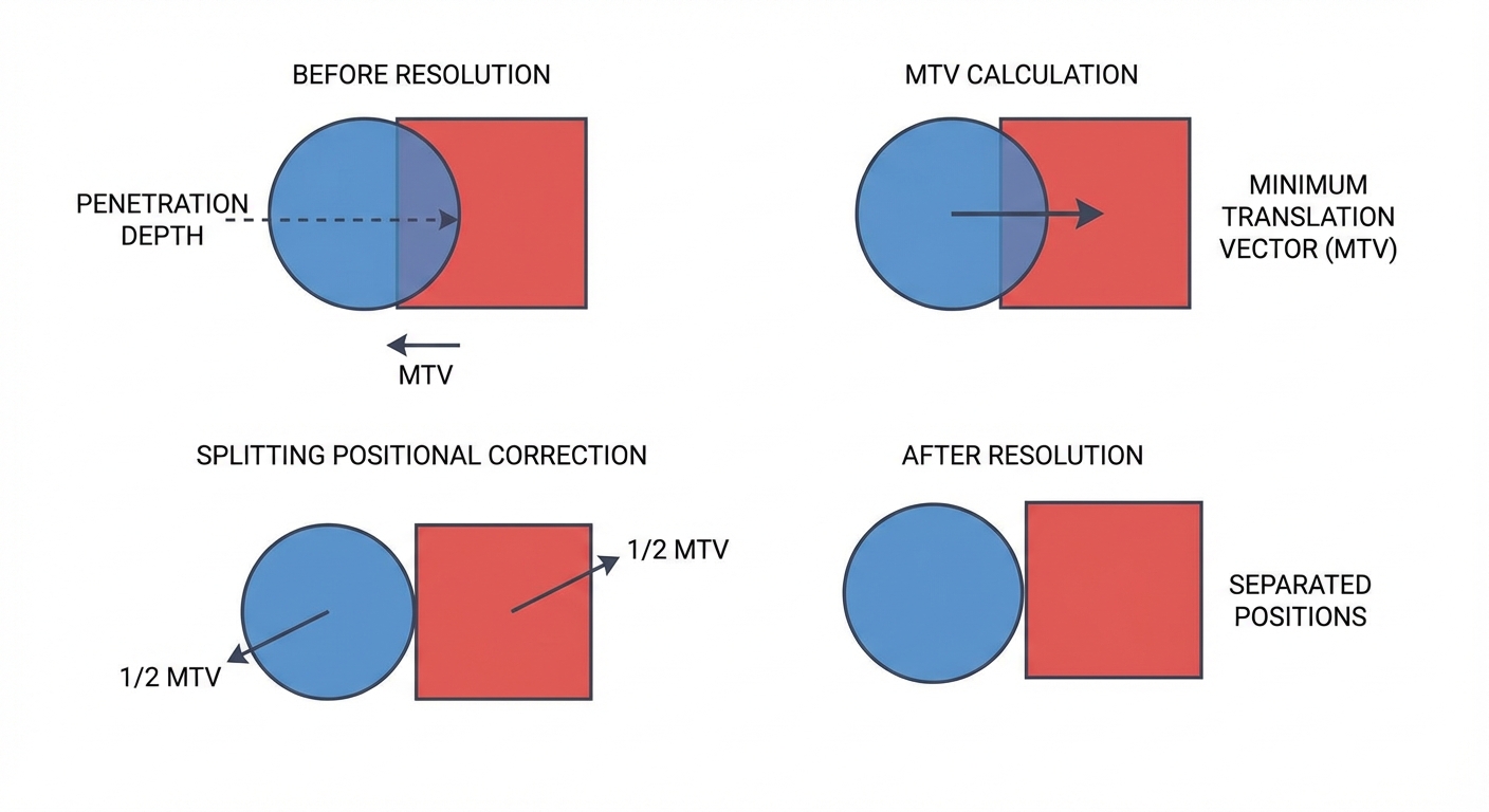
From detection to resolution: using the MTV

Once you have (normal, depth), you can do simple positional correction.

For example, if A and B are dynamic and you want to split correction evenly:

• move A by $\text{mtvA} \cdot 0.5$
• move B by $\text{mtvB} \cdot 0.5$

Then compute collision impulses for velocities (beyond SAT itself). SAT gives you a good contact normal and penetration depth; impulse resolution is a separate topic.

Complexity and performance

For polygons with $n$ and $m$ vertices:

• number of axes tested: $n + m$
• projecting A onto one axis costs $O(n)$, projecting B costs $O(m)$

So total work is:

More explicitly: $(n+m)$ axes, each axis costs $O(n+m)$ total projection work.

In practice with small convex polygons (boxes, hulls with < 16 vertices) this is very fast.

If you need more speed:

• broad-phase culling (AABB, spatial hashing, sweep-and-prune)
• caching transformed vertices and (optionally) edge normals per frame
• specialized support-point methods for some shapes

Common bugs checklist

• Not convex (SAT as described assumes convex; concave needs decomposition).
• Forgetting to test axes from both polygons.
• Degenerate edges (duplicate vertices) producing a zero normal.
• Mixing up “separating line” (a line) with “separating axis” (its normal direction).
• Inconsistent MTV sign convention (decide: does your MTV move A or B, and stick to it).
• No epsilon handling for contact → jittering or missed collisions.
• Axis deduplication with too-large epsilon → missed collisions for skinny shapes.

Summary

• SAT tests whether two convex shapes are separated along any candidate axis.
• For convex polygons, it’s sufficient to test edge normals from both shapes.
• Projection reduces 2D overlap to 1D interval overlap.
• Tracking the minimum overlap gives you an MTV: a normal and depth for collision resolution.

If you implement just one robust convex collision test for 2D, SAT is a strong choice.