How a Basic Rigid Body Simulation Works: Forces, Properties, and Stepping Forward in Time

Rigid body simulation is the workhorse behind most real-time physics in games and interactive tools. A rigid body is an object that does not deform: distances between points on the object remain constant. That simplification lets us describe motion using just a handful of state variables (position, orientation, velocities) and update them over time.

Who this is for (and what you’ll be able to implement)

If you’re building a small engine, a gameplay prototype, or a learning project and you want “an object that moves and spins when I push it,” this post is for you.

After reading, you should be able to implement:

• A single rigid body with force + torque accumulation
• A semi-implicit Euler time step
• A quaternion-based orientation update (first-order, with normalization)
• A fixed-timestep loop (with a catch-up cap)

Collisions/constraints are mostly out of scope, but I’ll point out where they typically fit into the step.

Conventions (so we don’t silently disagree)

Physics code is full of “looks right” bugs caused by mismatched conventions. Here are the assumptions in this post:

• Coordinate system: right-handed
• Spaces:
  • World space: global coordinates
  • Body (local) space: coordinates attached to the rigid body
• Angles: radians
• Units: SI-style (meters, kilograms, seconds) or any consistent set
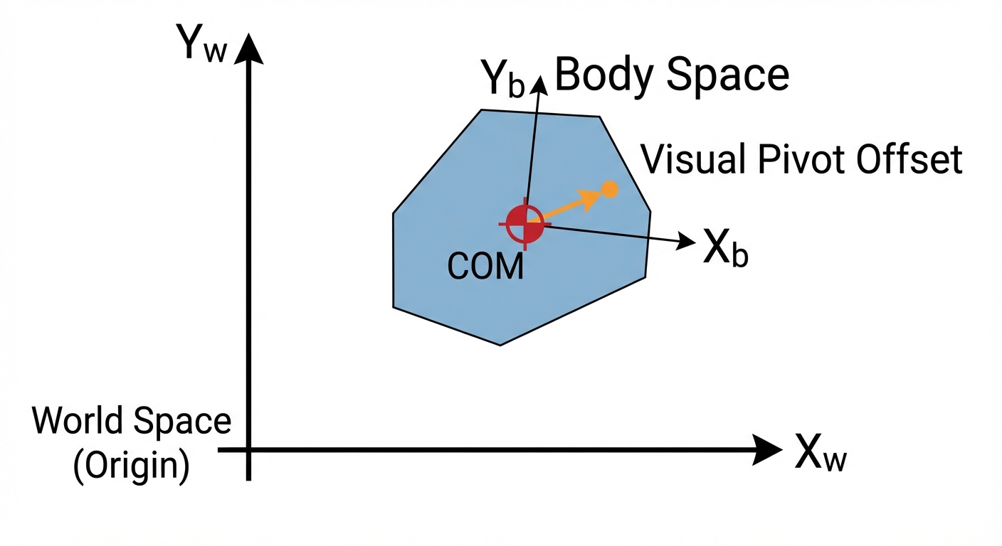
• Center of mass (COM): the state variables below (position/orientation) are defined at the center of mass

If your rendered mesh origin is not at the COM, you’ll need a fixed offset transform between the visual transform and the physical COM transform.

The basic loop

This post focuses on the “basic loop” of a rigid body simulator:

1. Store the body’s physical properties and state.
2. Accumulate forces and torques for the current frame.
3. Integrate (step forward in time) to update velocities and poses.
4. (Optionally) handle collisions/constraints.

Sanity check: if you apply no forces and no torques, both linear and angular velocities should remain constant (ignoring damping), so the body should coast and spin forever.

The state of a rigid body (at the center of mass)

A single rigid body in 3D typically tracks:

• Position: $\mathbf{x}$ (world-space center of mass)
• Orientation: $\mathbf{q}$ (often a quaternion)
• Linear velocity: $\mathbf{v}$ (world space)
• Angular velocity: $\boldsymbol{\omega}$ (we’ll treat this as world space in this post)

And physical properties:

• Mass: $m$ (or inverse mass $m^{-1}$)
• Inertia tensor: $\mathbf{I}$ (or inverse inertia) about the center of mass
• Damping (optional): linear and angular damping coefficients

Why store inverse mass/inertia? Because the “solve” step uses divisions a lot, and multiplying by inverse values is faster and numerically convenient. Also, static objects are naturally represented by setting inverse mass to 0.

COM vs. visual origin (important in practice)

All formulas that use $\mathbf{r} = \mathbf{p} - \mathbf{x}$ assume $\mathbf{x}$ is the center of mass. If your model’s pivot is elsewhere, you can still simulate correctly—just keep a constant offset from COM to render origin and apply it when drawing.

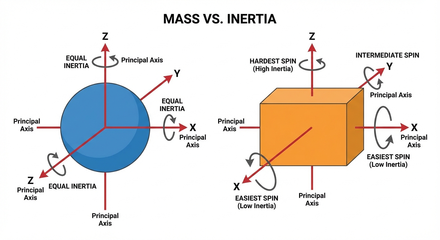
Mass vs. inertia (what they control)

• Mass controls how forces change linear motion:

• Inertia controls how torques change angular motion:

Key clarification: inertia is a tensor (a 3×3 matrix in 3D), and it depends on:

• the object’s mass distribution (shape + density)
• the reference point (here: COM)
• the chosen frame (body space vs world space)

Concrete intuition:

• A solid sphere has the same inertia in every direction → it’s equally easy to spin about any axis.
• A box is typically easier to spin about some axes than others (e.g., a long thin box is easiest to spin about its long axis and hardest about an axis that swings the long length around).

Sanity check: if you apply the same off-center push to a sphere and a long box of the same mass, you should see similar linear acceleration but potentially very different angular acceleration.

Inverse inertia: common storage pattern

A very common pattern is:

• Store $\mathbf{I}^{-1}_{body}$ in body space.
• Compute $\mathbf{I}^{-1}_{world}$ each step from the current orientation.

In body space, many shapes have inertia aligned with their principal axes, which makes $\mathbf{I}_{body}$ (and $\mathbf{I}^{-1}_{body}$) diagonal—cheap and stable.

Assumptions you’ll usually rely on:

• $\mathbf{I}$ is symmetric
• For dynamic bodies, $\mathbf{I}$ is positive definite (so the inverse exists)
• For static bodies, inertia is usually irrelevant because you won’t integrate them

Forces and torques

A rigid body responds to:

• Forces (change linear velocity)
• Torques (change angular velocity)

Common forces:

• Gravity: $\mathbf{F}_g = m\,\mathbf{g}$
• Springs, thrusters, drag, user inputs

Gravity: force vs. acceleration

You’ll commonly see gravity applied in either of these equivalent ways:

• As a force: $\mathbf{F} += m\,\mathbf{g}$ (then $\mathbf{a} = m^{-1}\mathbf{F}$)
• Directly as an acceleration: $\mathbf{a} += \mathbf{g}$

This post’s loop uses force accumulation, so gravity is typically added as $\mathbf{F} += m\,\mathbf{g}$. If you only store invMass, you can compute $m$ as $1/\text{invMass}$ for dynamic bodies, or just add gravity as acceleration instead.

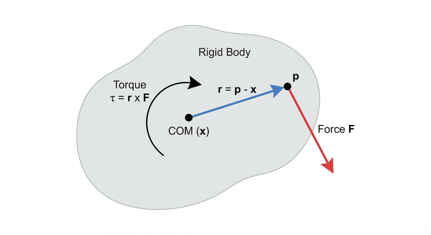
Applying a force at a point produces torque

If you apply a force $\mathbf{F}$ at a world-space point $\mathbf{p}$, not necessarily at the center of mass $\mathbf{x}$, you get:

• Net force adds to linear motion: $\mathbf{F}_{net} += \mathbf{F}$
• Net torque adds to angular motion:

If the force is applied at the center of mass, $\mathbf{r}=\mathbf{0}$ and there is no torque.

Force accumulators

A common pattern is to accumulate forces and torques over the frame:

• $\mathbf{F}_{net}$: starts at zero each step
• $\boldsymbol{\tau}_{net}$: starts at zero each step

Then, after integration, clear them (or clear them at the start of the next step—just do it once per step, consistently).

This makes it easy to have multiple systems contribute forces (gravity, input, buoyancy, etc.) without them fighting over the body state.

Sanity check: applying a force at the COM should change $\mathbf{v}$ but not $\boldsymbol{\omega}$. Applying equal and opposite forces at different points (a “couple”) should produce torque with near-zero net force.

From forces to accelerations (keep spaces consistent)

At each step, compute accelerations:

• Linear acceleration (world space):

• Angular acceleration:

Important: $\boldsymbol{\omega}$, $\boldsymbol{\tau}$, and $\mathbf{I}^{-1}$ must be expressed in the same space.

In this post we’ll use:

• $\boldsymbol{\omega}$ in world space
• $\boldsymbol{\tau}$ in world space (because $\mathbf{r} \times \mathbf{F}$ is computed in world space)
• $\mathbf{I}^{-1}_{world}$ to match

World-space inertia (and what $\mathbf{R}$ means)

Most inertia tensors are easiest to define in the body’s local space (aligned with the shape). But torques and angular velocities are often handled in world space.

Let:

• $\mathbf{I}_{body}$ be inertia in body space
• $\mathbf{R}$ be the 3×3 rotation matrix corresponding to the current orientation quaternion $\mathbf{q}$
• $\mathbf{R}$ maps body → world for vectors

Then:

and similarly for the inverse:

This form avoids matrix-order ambiguity if you remember: rotate into world, apply, rotate back.

Sanity check: if the body rotates 90° in world space, the inertia “seen in world axes” should rotate with it (so the response to the same world-space torque can change as the object turns).

Stepping forward in time (integration)

“Integration” is how we update velocities and poses using accelerations over a small timestep $\Delta t$.

A typical rigid body update has two parts:

1. Update velocities from accelerations.
2. Update position/orientation from velocities.

Where do collisions/constraints go? Commonly:

• Integrate external forces into velocities
• Solve constraints / collision impulses to modify velocities
• Integrate pose from the final velocities

(That’s one common arrangement; engines differ, but this is a useful mental model.)

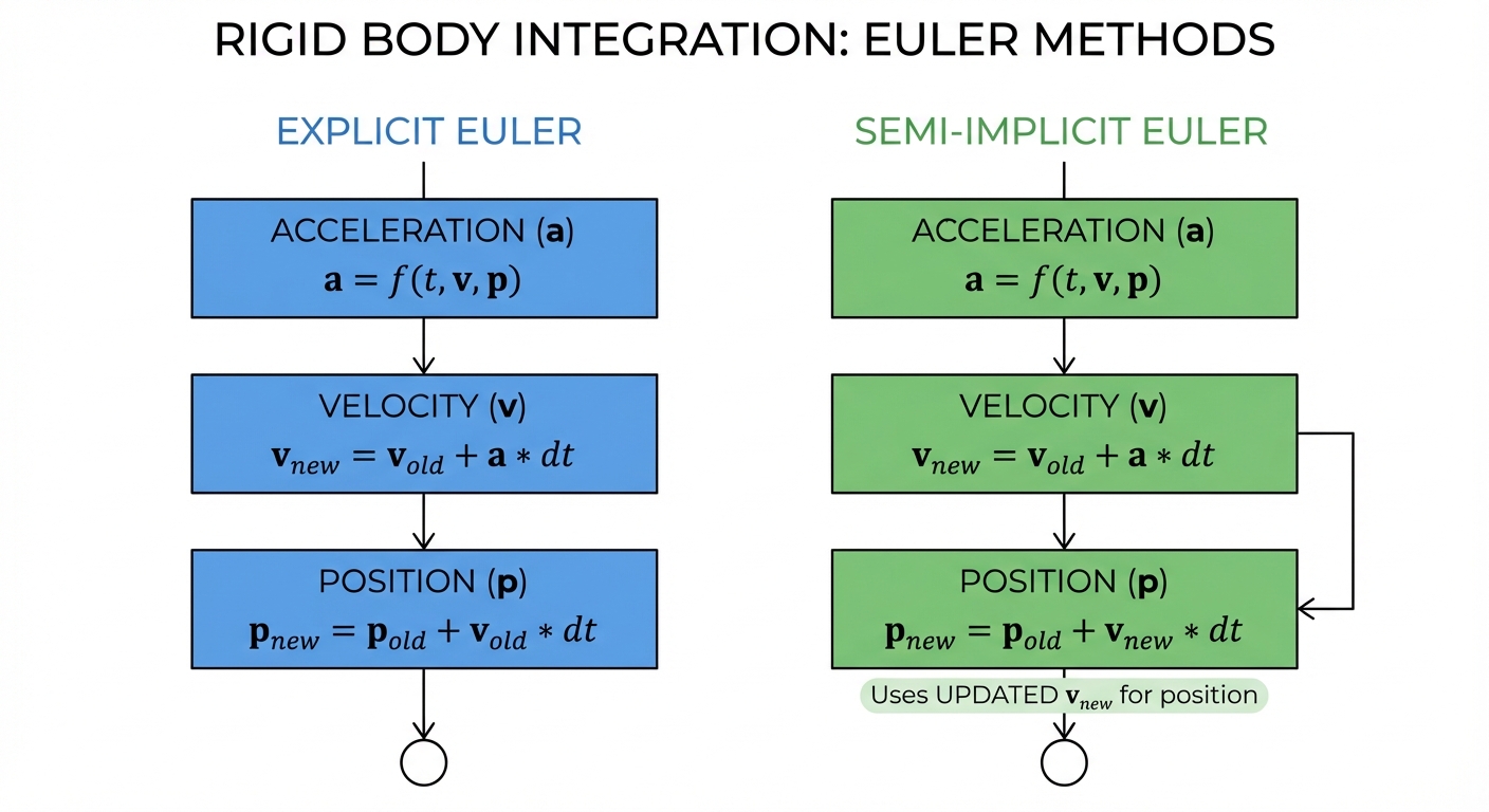
Semi-implicit Euler (a good basic choice)

The simplest integrator is explicit Euler, but for physics it can be unstable (energy can blow up). A common “basic but better” option is semi-implicit Euler (a.k.a. symplectic Euler):

1. Update velocities:

2. Update pose using the new velocities:

Orientation update is a bit more involved; see below.

Sanity check: with constant gravity and no other forces, vertical velocity should change linearly over time and position should follow a parabola.

Updating orientation with angular velocity (quaternion convention)

Quaternion kinematics are convention-dependent. Here’s the convention used in this post:

• $\mathbf{q}$ rotates vectors from body → world.
• $\boldsymbol{\omega}$ is the angular velocity in world space.
• Quaternion derivative uses right-multiplication by the angular-velocity quaternion:

Let $\boldsymbol{\omega}_q = (0, \omega_x, \omega_y, \omega_z)$. Then:

A simple first-order (Euler) quaternion integration is:

Finally, normalize the quaternion to prevent drift:

This is a first-order orientation integrator: it works well with small $\Delta t$ and normalization. More accurate options exist (e.g., exponential map / integrating with $\Delta q$), but you don’t need them to get a solid basic simulator.

Sanity check: if $\boldsymbol{\omega} = \mathbf{0}$, orientation should not change. If $\boldsymbol{\omega}$ is constant, the body should spin at a steady rate.

Damping (stability + a bit of realism)

Real systems lose energy due to friction and air resistance. In simulations, damping also helps prevent jitter and numerical runaway.

It’s common to apply damping after you’ve integrated velocities (and after any constraint/collision velocity corrections), because it acts like a stabilizing “drag” on the final velocities.

A robust way to express damping is exponential decay:

• $\mathbf{v} \leftarrow \mathbf{v}\,e^{-k_{lin}\,\Delta t}$
• $\boldsymbol{\omega} \leftarrow \boldsymbol{\omega}\,e^{-k_{ang}\,\Delta t}$

If you prefer the $(1-d)^{\Delta t}$ form:

• Ensure $d \in [0,1)$
• Interpret $d$ consistently (per-second vs per-step)
• Clamp to avoid $1-d \le 0$ causing pow() issues

Sanity check: with damping enabled and no forces, speeds should monotonically decrease toward zero (never grow).

Putting it together: the minimal simulation loop

Below is a compact “single body” view. A real engine loops over all bodies.

One clean ordering is:

1. Clear accumulators (start-of-step)
2. Add forces/torques (gravity, controls, etc.)
3. Compute accelerations
4. Integrate velocities
5. (Optional) solve collision/constraint impulses on velocities
6. Apply damping
7. Integrate pose (position + orientation)

You can swap steps 6 and 7 (many do), but keep the ordering consistent.

Pseudocode

struct RigidBody {
  Vec3 x;          // world position of center of mass
  Quat q;          // orientation (body -> world)

  Vec3 v;          // linear velocity (world)
  Vec3 omega;      // angular velocity (world, radians/sec)

  float invMass;   // 0 for static
  Mat3 invInertiaBody; // body-space inverse inertia (often diagonal)

  Vec3 force;      // accumulated force (world)
  Vec3 torque;     // accumulated torque (world)

  float linDamp;   // >= 0 (interpreted as k in exp(-k*dt))
  float angDamp;   // >= 0
};

void clearAccumulators(RigidBody& b) {
  b.force  = Vec3(0,0,0);
  b.torque = Vec3(0,0,0);
}

void applyForceAtPointWorld(RigidBody& b, Vec3 F_world, Vec3 p_world) {
  b.force += F_world;
  Vec3 r_world = p_world - b.x;      // lever arm from COM
  b.torque += cross(r_world, F_world);
}

void applyGravityAsForce(RigidBody& b, Vec3 g_world) {
  if (b.invMass == 0.0f) return;
  float mass = 1.0f / b.invMass;
  b.force += mass * g_world;
}

void step(RigidBody& b, float dt) {
  if (b.invMass == 0.0f) return; // static body: skip integration

  // Clamp damping inputs for robustness
  float kLin = max(0.0f, b.linDamp);
  float kAng = max(0.0f, b.angDamp);

  // 1) linear acceleration (world)
  Vec3 linAcc = b.force * b.invMass;

  // 2) angular acceleration (world)
  // R is the rotation matrix for q (body -> world)
  Mat3 R = toMat3(b.q);
  Mat3 invInertiaWorld = R * b.invInertiaBody * transpose(R);
  Vec3 angAcc = invInertiaWorld * b.torque;

  // 3) integrate velocities (semi-implicit Euler)
  b.v     += linAcc * dt;
  b.omega += angAcc * dt;

  // 4) optional: collision/constraint impulses would typically modify b.v/b.omega here

  // 5) damping (exponential form)
  b.v     *= exp(-kLin * dt);
  b.omega *= exp(-kAng * dt);

  // 6) integrate position
  b.x += b.v * dt;

  // 7) integrate orientation (world-space omega convention)
  Quat omegaQ(0, b.omega.x, b.omega.y, b.omega.z);
  Quat dq = 0.5f * (omegaQ * b.q);
  b.q += dq * dt;
  b.q = normalize(b.q);

  // 8) clear accumulators (end-of-step)
  clearAccumulators(b);
}

Notes:

• If rotation is locked (or invInertiaBody is zero), you can skip the inertia transform and angular integration.
• For static bodies (invMass = 0), inertia is typically irrelevant because you don’t integrate them.

Choosing a timestep: fixed vs. variable

Your integrator assumes $\Delta t$ is “small enough.” If $\Delta t$ varies wildly, stability suffers.

• Fixed timestep (e.g., 1/60 s) is common for physics.
• If rendering is variable, use an accumulator:
  • Add frame time to an accumulator
  • Step physics in fixed increments while accumulator ≥ dt
  • Optionally interpolate for rendering

Actionable detail: cap your catch-up to avoid the “spiral of death” when the game hitches.

• Limit max accumulated time (e.g., clamp accumulator to 0.25 s)
• Or limit max substeps per frame (e.g., 4–8)

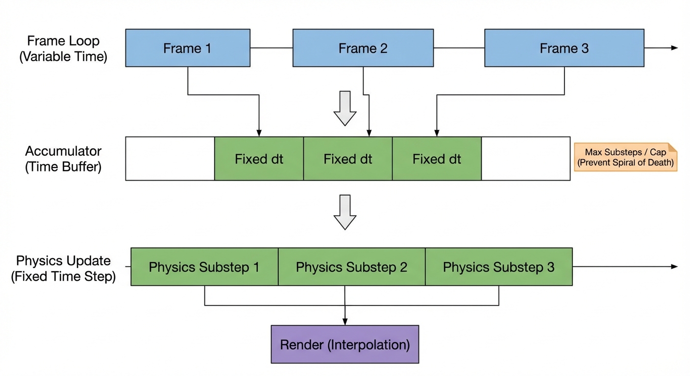
Sanity check: if the frame rate drops, physics should slow down gracefully (or temporarily lose accuracy), not explode due to a huge dt.

Common pitfalls (worth checking before you debug for hours)

• Forgetting to normalize quaternions (orientation slowly breaks)
• Mixing degrees and radians for $\boldsymbol{\omega}$
• Mixing world space and body space for $\boldsymbol{\tau}$, $\boldsymbol{\omega}$, and $\mathbf{I}^{-1}$
• Applying torque with the wrong lever arm (not using COM)
• Using a highly variable $\Delta t$ without a fixed-step accumulator
• Damping parameters that imply invalid math (negative values, or using $(1-d)^{dt}$ with $d\ge 1$)

What we didn’t cover (but your simulator will need next)

A force-and-integrate loop produces motion, but a “physics engine” usually adds:

• Collision detection (broad phase + narrow phase)
• Contact constraints (prevent interpenetration, add friction)
• Joints/constraints (hinges, sliders, distance constraints)
• Sleeping (stop simulating bodies at rest)

Those pieces typically work by computing impulses or constraint forces that modify velocities during the step (often after external forces are applied and before integrating pose).

Summary

A basic rigid body simulation boils down to:

• Store state at the center of mass: $\mathbf{x}, \mathbf{q}, \mathbf{v}, \boldsymbol{\omega}$
• Store properties: inverse mass and inverse inertia (commonly $\mathbf{I}^{-1}_{body}$)
• Accumulate forces and torques
• Convert them to accelerations (in consistent spaces)
• Integrate velocities and then pose (semi-implicit Euler is a solid starting point)
• Normalize orientation and apply damping
• Prefer a fixed timestep (with a catch-up cap) for stability

Once you have this loop working, you have the foundation needed to add collisions, constraints, and more realistic interactions.