Collision detection in 3D is the problem of deciding whether two objects occupy any common volume, whether their surfaces touch, or how far apart they are—depending on what you ask for. It shows up everywhere: games, robotics, CAD, simulation, and AR/VR.
Target reader: engineers implementing or choosing collision techniques in a real-time system (game/robotics/simulation). The math is kept lightweight, with pointers to canonical references.
What you’ll learn / when to use which (in 60 seconds):
- How real systems combine broad phase → narrow phase → contact generation for performance.
- Which narrow-phase family to pick: primitives, convex (SAT/GJK+EPA), or meshes (BVH + triangle tests).
- When you need boolean intersection vs distance vs penetration/contacts vs continuous collision detection (TOI).
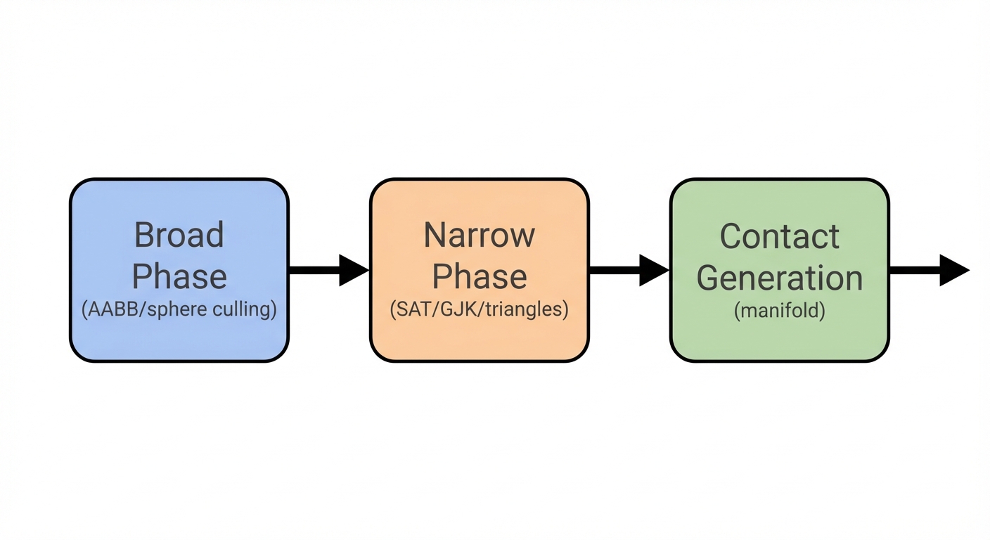
Most real systems don’t use a single “perfect” test. Instead, they use a pipeline:
- Broad phase: quickly rule out most pairs using cheap approximations.
- Narrow phase: run an exact or higher-fidelity test on the remaining candidates.
- Contact generation (optional but common): compute contact points, normals, and penetration depth for physics.
See Fig. 1 for the typical pipeline structure.
Tighten terminology: intersection, touching, distance
Before choosing an approach, be explicit about the query you need.
- Volume intersection (overlap): do the interiors overlap? (boolean)
- Surface contact (touching): do the boundaries just touch? (boolean, but sensitive to tolerance)
- Distance query: what is the minimum separation distance if not intersecting? (nonnegative scalar)
- Penetration depth: how deep are they overlapping if intersecting? (nonnegative scalar)
- Contacts / manifold: where to apply forces (points), in which direction (normal), and with what depth.
In practice, engines usually treat “touching counts as collision” because of finite precision and solver stability. That means comparisons are often inclusive (e.g., ) with a small tolerance .
Capability map: what each method gives you
A useful way to organize algorithms is by what they naturally return.
- Boolean-only (fast): AABB/OBB overlap, many primitive tests, triangle-triangle (boolean).
- Distance queries (useful for planning/CCD): point–segment, segment–segment, GJK (distance variant), SDF (approximate unless conservative).
- Penetration + contacts (physics): SAT (penetration axis), GJK+EPA (depth/normal), plus contact manifold generation (separate step).
Broad-phase approaches (fast culling)
Broad phase aims to cheaply reject most object pairs. It trades accuracy (false positives) for speed.
Axis-Aligned Bounding Boxes (AABB)
An AABB is defined by min/max coordinates along world axes: , , .
Two AABBs overlap iff they overlap on all three axes. On x:
- inclusive (touching counts): and
- exclusive (touching does not count): and
In real-time physics, you’ll often use an epsilon to avoid jitter:
- “treat as overlap if within tolerance”: (and symmetric)
Fig. 2 illustrates why AABBs can produce false positives under rotation.
Pros:
- Extremely fast (just comparisons)
- Easy to update for translating objects
Cons:
- Loose fit for rotated objects (can over-report collisions)
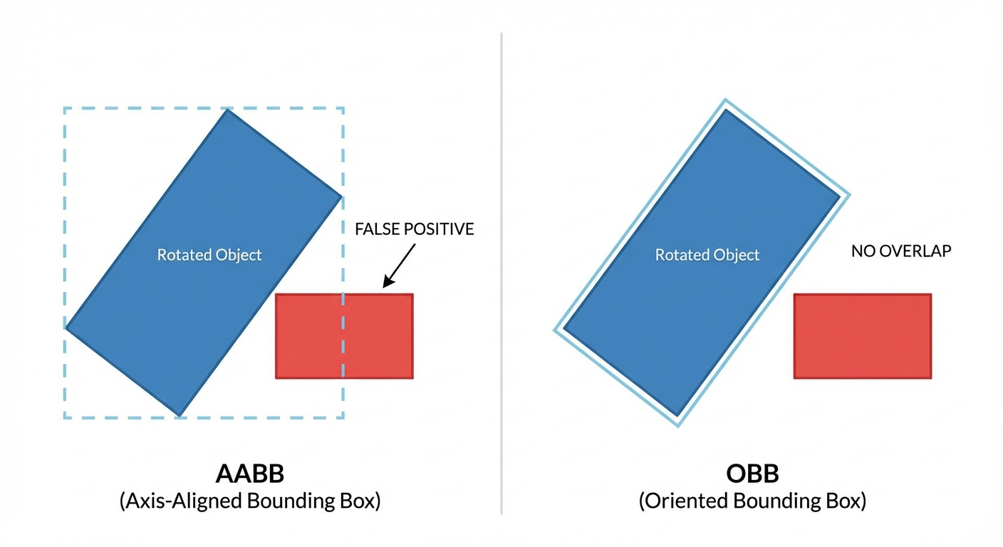
Oriented Bounding Boxes (OBB)
An OBB is an AABB in the object’s local frame, rotated with the object. It fits tighter than an AABB for rotated shapes.
A common test is Separating Axis Theorem (SAT) specialized for boxes. For two OBBs, you test up to 15 axes:
- 3 face normals of box A:
- 3 face normals of box B:
- 9 cross-product axes: for
Practical optimization: if is near zero (edges nearly parallel), that axis is numerically unstable and often redundant—skip it using a small threshold.
Pros:
- Much tighter than AABB
Cons:
- More expensive than AABB
- Implementation complexity is higher
Bounding spheres
A sphere is defined by center and radius . Two spheres overlap if:
Pros:
- Rotation-invariant
- Very cheap
Cons:
- Often a poor fit (lots of false positives)
Spatial partitioning (reduce pair counts)
Instead of testing every pair, partition space so you only test nearby objects.
Common choices:
- Uniform grids / spatial hashing: great when object sizes are similar.
- Sweep-and-prune (sort-and-sweep): common in engines; exploits temporal coherence of AABB endpoints.
- Octrees: adapt to varying densities.
- Scene-level BVH: hierarchical culling across many objects.
These methods don’t replace overlap tests; they reduce how many you need.
Narrow-phase approaches (accurate tests)
Once a pair survives broad phase, narrow phase determines overlap more precisely.
Convexity callout: SAT and GJK assume convex shapes. For concave shapes, you typically use convex decomposition or a mesh BVH / triangle-level method (or both).
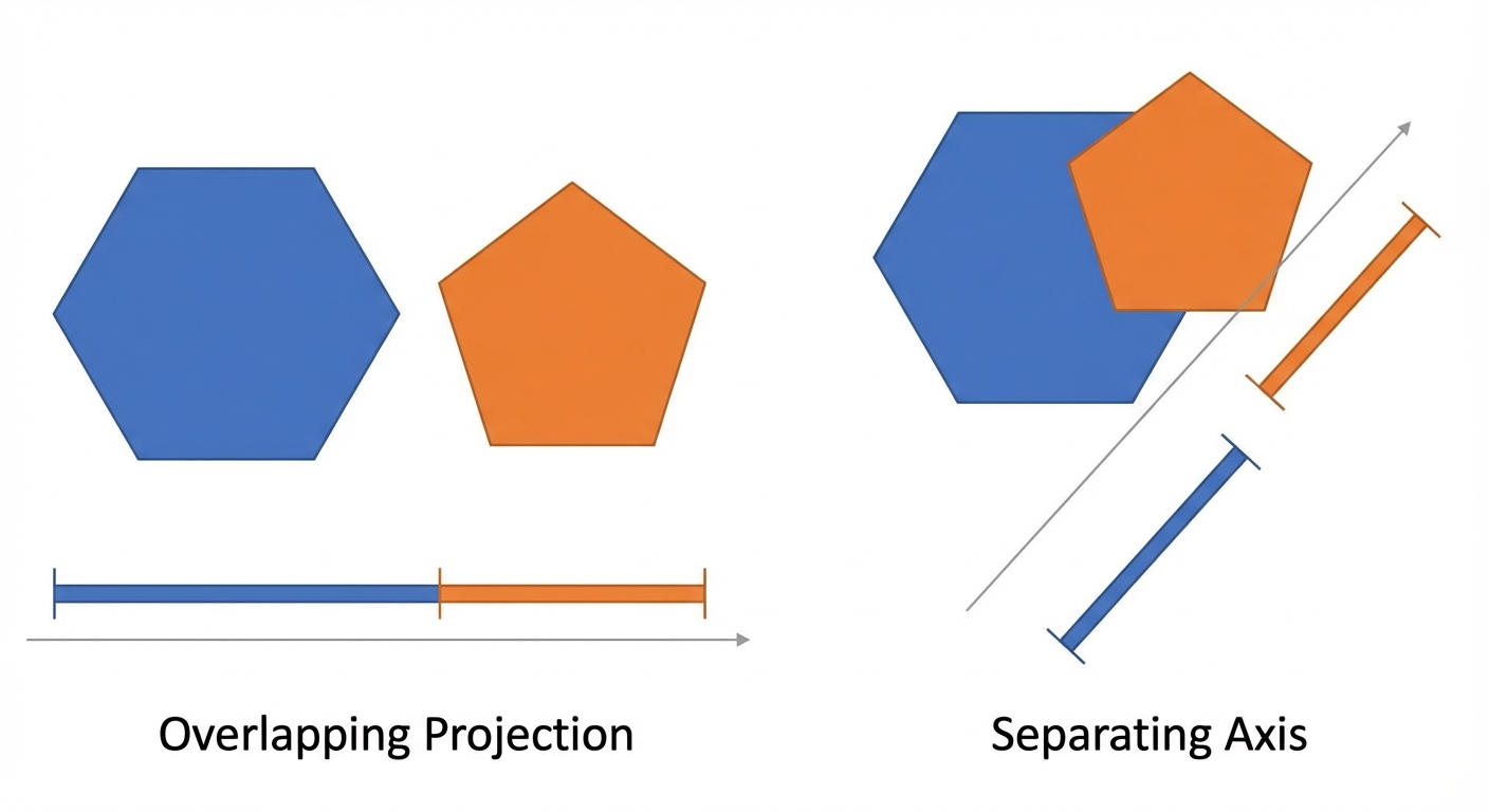
Separating Axis Theorem (SAT) for convex polyhedra
SAT is a workhorse for convex collision detection.
Key idea: Two convex shapes do not overlap iff there exists an axis along which their projections are disjoint.
For convex polyhedra, candidate separating axes come from:
- Face normals of both shapes
- Cross products of edges from shape A with edges from shape B
Let be a unit axis (normalize it). Project a vertex onto it with scalar projection:
Compute intervals and . If they are disjoint, you found a separating axis → no collision.
If they overlap on all tested axes, the shapes intersect. The minimum-overlap axis is often used as an estimate of penetration direction and depth.
Cost drivers: number of faces and (especially) edge pairs. Common accelerations:
- Precompute face normals and unique edge directions.
- Use adjacency information to avoid redundant edge cross-products.
- Exploit temporal coherence: cache the last separating axis (or best axis) and test it first next frame.
Fig. 3 visualizes projections and the “gap” that proves separation.
Pros:
- Exact for convex shapes
- Can be extended to compute penetration depth (minimum overlap axis)
Cons:
- Requires enumerating candidate axes (can be many)
- Not directly applicable to concave shapes without decomposition
GJK (Gilbert–Johnson–Keerthi) for convex shapes
GJK determines whether two convex shapes intersect by working in the Minkowski difference:
The shapes intersect iff the origin lies inside .
GJK doesn’t build the Minkowski difference explicitly. It only needs a support function for a convex set :
For the Minkowski difference:
What the simplex means: GJK maintains a simplex (point/line/triangle/tetrahedron in 3D) whose vertices are support points of . If the simplex can be expanded to contain the origin, the shapes intersect. Termination typically occurs when:
- the simplex contains the origin (intersection), or
- the closest point on the simplex to the origin stops improving beyond a tolerance (no intersection / distance found).
Common failure modes: degeneracy (nearly collinear/coplanar support points), cycling, and floating-point noise. Practical implementations use:
- iteration caps,
- tolerances on improvement,
- simplex “cleanup” rules,
- and often warm-starting (initialize direction/simplex from the previous frame).
Pros:
- Very fast in practice for convex shapes
- Works with any convex shape that has a support mapping (spheres, capsules, convex hulls)
Cons:
- Often implemented as boolean; distance/closest features require careful variant
- For penetration depth you typically pair it with EPA
EPA (Expanding Polytope Algorithm) for penetration depth
If GJK reports intersection, EPA expands the simplex into a polytope approximating the boundary of and finds the closest face to the origin. This yields, in Minkowski space:
- a penetration normal direction,
- a penetration depth magnitude.
World-space outputs:
- The normal is used as the contact normal in world space (after consistent orientation).
- The depth is a scalar along that normal.
- A contact point is typically derived by tracking the corresponding support points on A and B for the closest Minkowski face (and then computing witness points). Note: this single point is not a stable manifold by itself.
Robustness issues: numerical error can make the polytope inconsistent (non-manifold faces, tiny triangles). Typical mitigations:
- face/edge cleanup and duplicate removal,
- minimum area/angle thresholds,
- fallback to a simpler contact estimate when EPA fails.
Pros:
- Common pairing with GJK in physics engines
Cons:
- More complex; needs robust handling for degeneracies
Primitive-vs-primitive tests (fast and exact)
Many engines represent collision shapes as primitives because the math is stable, cheap, and easy to make robust.
Common exact tests include sphere–sphere, sphere–capsule, capsule–capsule, box–sphere, and box–box (often SAT-optimized). Below are two non-trivial distance kernels that show up everywhere.
Point–segment distance (sphere–capsule core)
Given point and segment endpoints . Let .
Compute parameter:
Clamp to , then closest point is . Distance is .
Sphere–capsule intersects if (with capsule radius included).
Segment–segment distance (capsule–capsule core)
Given segments and with .
You solve for that minimize (a small 2×2 system), then clamp to with case handling for parallel segments.
Capsule–capsule intersects if the segment–segment distance is .
(For a canonical, robust derivation, see Ericson.)
Mesh collisions: triangle-level approaches
When objects are arbitrary triangle meshes, you typically rely on hierarchies to avoid triangle checks.
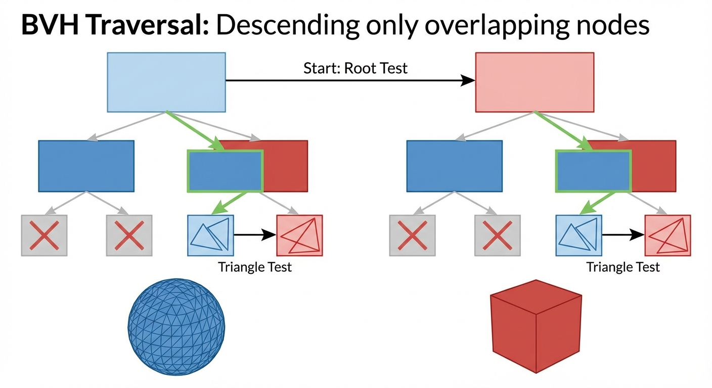
BVH (Bounding Volume Hierarchy)
A BVH is a tree where each node bounds a subset of triangles (often with AABBs, but OBBs and k-DOPs are also used). To test two meshes:
- Test root volume vs root volume.
- If they overlap, descend into children.
- Only when you reach leaf nodes do you run triangle-triangle intersection tests.
Fig. 4 shows how BVH traversal prunes most triangle pairs.
Pros:
- Scales well
- Works for general meshes
Cons:
- Needs building/updating; dynamic meshes require refitting or rebuilding
Refit vs rebuild (important in practice):
- Refit: update node bounds to enclose moved triangles without changing topology. Good when the mesh undergoes a rigid transform or small deformations. Fast, but tree quality can degrade over time.
- Rebuild: reconstruct the BVH (e.g., SAH-based). More expensive, but restores good culling. Used for large deformations or when refit becomes too loose.
Triangle–triangle intersection (leaf test)
At the leaf level, you test whether two triangles intersect.
Be explicit about the predicate you need:
- Proper intersection: interiors intersect (excluding purely coplanar overlap).
- Including coplanar overlap: counts coplanar edge/area overlap as intersection.
Robust implementations prefer geometric predicates (orientation tests) over ad-hoc epsilons, especially for near-coplanar cases. A widely cited reference is Möller’s triangle-triangle intersection work.
If you only need a boolean, triangle-triangle tests may be enough. For physics contacts, you usually need additional processing to produce stable contact manifolds.
Signed Distance Fields (SDF) for overlap/distance queries
An SDF returns signed distance to a surface: negative inside, positive outside. SDFs are great for distance queries and smooth effects, but you should treat sampling-based overlap tests as approximate unless you use conservative bounds.
What’s reliable:
- Querying the SDF at a point gives a distance estimate (quality depends on representation).
What’s not automatically reliable:
- “If any sampled point from B has then overlap” can miss collisions due to aliasing, thin features, and insufficient sampling density.
Practical notes:
- Many systems use narrow-band SDFs (store distances only near the surface) to reduce memory.
- Resolution controls accuracy; thin features smaller than a voxel can disappear.
- For conservative collision, combine SDFs with bounding volumes, Lipschitz bounds, or guaranteed sampling strategies.
Pros:
- Great for smooth distance queries and effects (soft bodies, VFX)
Cons:
- Memory/compute cost; exactness depends on representation and conservativeness
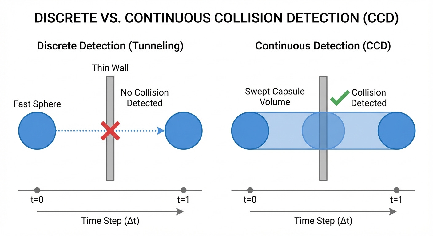
Continuous Collision Detection (CCD): avoid tunneling
Discrete collision detection checks overlap at fixed time steps. Fast-moving objects can “tunnel” through each other between frames.
It helps to distinguish three approaches:
- Discrete: test only at end-of-step (or start/end). Fast, but can miss collisions.
- Speculative contacts: predict likely contacts using inflated shapes or motion bounds, then let the solver prevent penetration. Often cheaper than true TOI, but can be conservative.
- True TOI (time of impact): compute whether objects overlap at any during the step, and find the earliest collision time.
Common CCD strategies:
- Swept volumes: e.g., a moving sphere over a step becomes a capsule; test that against the target.
- TOI solvers: root-finding on distance functions.
- Conservative advancement: advance time by a safe amount based on current separation and relative speed.
Concrete anchor example (sphere vs triangle TOI): treat the sphere center as moving along a segment and solve for the earliest where distance to the triangle equals the radius (often by considering triangle features: face, edges, vertices).
Fig. 5 illustrates tunneling and the swept-volume idea.
Practical selection guide (decision table)
Use this as a starting point; real engines mix rows.
| Shape types | Motion | Required output | Typical choice |
|---|---|---|---|
| Many rigid bodies (primitives/convex) | Dynamic | Boolean + contacts | Broad: AABB + sweep-and-prune/hash; Narrow: primitives or GJK+EPA; Contacts: manifold generation |
| Convex shapes (planning/optimization) | Dynamic | Distance (and gradients) | GJK distance variant; cache/warm-start for temporal coherence |
| Complex static environment (mesh) vs dynamic actors | Mostly static | Boolean/contacts | Static mesh BVH (AABB/OBB/k-DOP); dynamic proxies as primitives/convex |
| Concave rigid meshes | Dynamic | Boolean/contacts | Per-object BVH + triangle tests; or convex decomposition + GJK |
| Very fast motion | Dynamic | TOI | CCD: swept primitives, conservative advancement, or dedicated TOI per pair |
Contact generation and manifold stability (physics engines)
Penetration depth and a single normal (from SAT or EPA) are usually not enough for stable stacking and friction.
Engines typically build and maintain a contact manifold:
- multiple contact points (up to 4 for box-like contacts is common),
- persistent across frames (keep IDs / feature pairs),
- updated with clipping/reduction,
- used with warm starting in the solver (reuse last frame’s impulses).
This is why “a contact point from EPA” is often treated as an input to a manifold builder rather than the final answer.
Performance notes (why caching matters)
- Broad phase: aims to reduce candidate pairs from toward near-linear in typical scenes via partitioning and coherence.
- Narrow phase scaling: SAT cost grows with faces/edges; BVH traversal cost depends on overlap and tree quality.
- Temporal coherence: reuse last frame’s information:
- last separating axis for SAT,
- warm-start direction/simplex for GJK,
- coherent BVH traversal and persistent pairs in broad phase.
Common pitfalls (and how to mitigate them)
- Floating-point tolerances: treat “almost touching” as contact using ; be consistent across broad/narrow/solver.
- Inclusive vs exclusive comparisons: decide whether touching counts as overlap; inclusive is common for stability.
- Poor bounding volumes: overly loose bounds cause too many narrow-phase calls.
- Concave shapes: use convex decomposition, voxel/SDF representations (with accuracy caveats), or mesh BVHs.
- Degenerate geometry: zero-area triangles, tiny edges; clean input or add robust predicate handling.
- Performance cliffs: worst-case SAT axes or deep BVH traversal; add caching, coherence, and good BVH maintenance (refit vs rebuild).
Summary
To detect whether two 3D objects overlap, you typically combine:
- Broad phase: AABB/spheres + sweep-and-prune/spatial hashing to find likely pairs
- Narrow phase:
- SAT or GJK(+EPA) for convex shapes (with convexity assumptions)
- BVH + triangle tests for meshes (with refit/rebuild strategy)
- SDFs for distance-style queries (often approximate unless conservative)
- CCD/TOI when motion between frames matters
- Contact manifold generation for stable physics (persistence, reduction, warm starting)
Choosing the right approach depends on shape types (primitive/convex/mesh), motion (static/dynamic/fast), and whether you need a boolean answer, distance, or stable contacts.
References / next steps
- Christer Ericson, Real-Time Collision Detection (broad phase, primitives, distance kernels)
- Gino van den Bergen, Collision Detection in Interactive 3D Environments (GJK and practical details)
- Tomas Möller, triangle-triangle intersection references (robust triangle tests)
- Bullet Physics (GJK/EPA, broadphase variants) and Box2D (2D but excellent broadphase/solver concepts)